
haystack-errw-proof
most inefficient method to find a needle in a haystack.
proof for why edge reinforced random walk, with a linear increment has a compute complexity of O(4n)i
visualization:
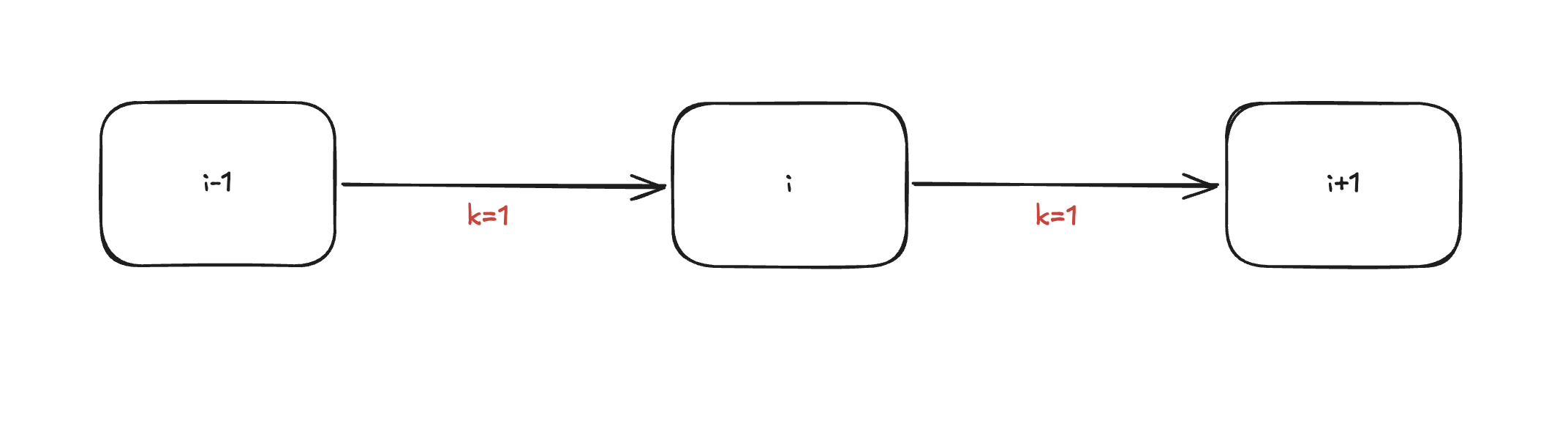
imagine you start at a random vertex, i. the odds you go to the left or to the right is based on the weight(k) of the edges, in between the bordering vertices.
say you flip a coin, its heads, and then you go to the right. now you are at vertex i+1 and the weight of the edge you just crossed is k=2:
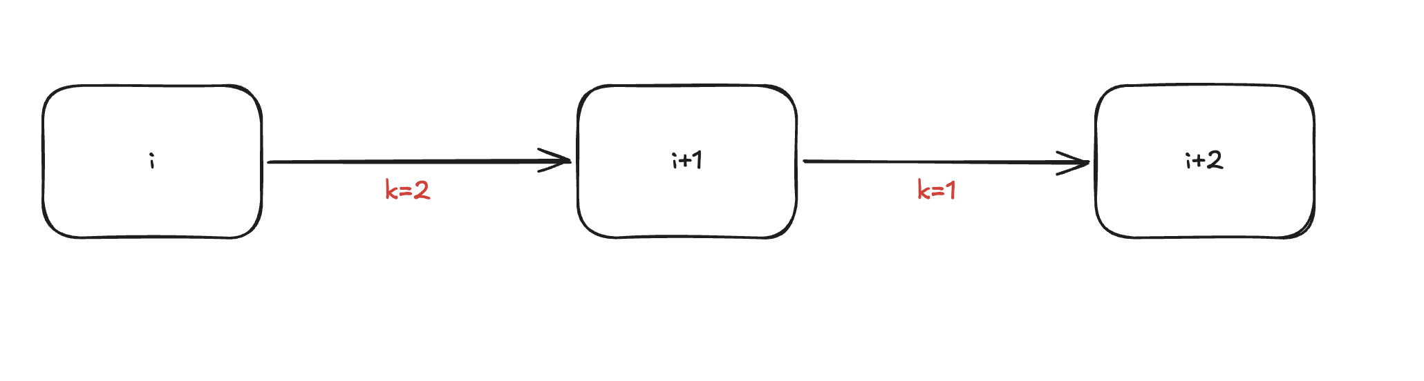
below is the proof for compute complexity of this method.
throughout this doc, log = natural log (base e).
1. get the relationship between total steps and the number of times you cross edge {i, i+1} to reach needle.
we can just track rightward crossings, and get leftward crossings based on it. we know that rightward crossings will always be 1 more than left, since we have to eventually get to vertex n.
so:
- Ri = rightward
- Ri-1 = leftward
so to get total number of crossings for edge i, its:
Ri + Ri-1 = 2Ri - 1
so we can represent the total number of crossings for every single edge with this summation:
2. find representation of a fixed probability we reach a given vertex
since we are at vertex i, we will start out with:
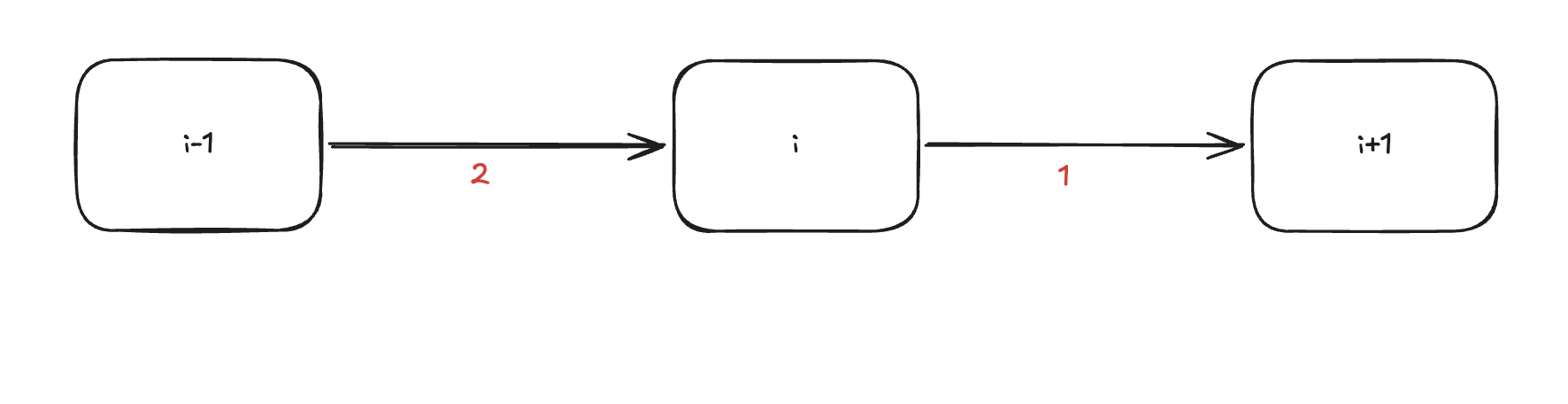
- edges are identified based on the vertex to the left of it.
- e.g. edge i has a value of 1, edge i-1 has a value of 2
the probability we visit vertex i+1 is essentially a polya urn problem. where you reach into a jar with a number of red balls, and b number of blue balls. whichever ball you draw, you place back in, and also reinforce its weight with an additional ball of the same color.
polya urn traditionally uses a beta distribution to represent the fixed probability we draw a blue ball on each attempt:
- Pi ~ Beta distribution(a, b)
beta distribution is the spread of possible values that Pi could be(between 0 and 1). we then randomly select a value from that spread to represent pi. this "randomly selected" value is a limit that is approached as number of attempts approach infinity.
- the limit here depends on random chance, thats why it is "random".
- it will not reach the same limit each time.
in theory we could increment the dials by 1 whenever they are drawn. but the whole point of the distribution is we can randomly calculate a fixed probability that we draw blue:
- say we have beta(1,1), the starting point of urn.
- we randomly get 0.3, meaning each attempt is a 30% chance of drawing blue. across many draws the proportion of blue balls will converge on 30%.
for our scenario, we can use beta for the success rate of vertex i+1 being visited. given you are at vertex i, and just passed through vertex i-1 once, the edge on the left will have additional weight.
by default polya urn increments the route chosen by 1. in our case, the weight of the edge increases by 2 for every departure (since you will leave to go to i-1, and cross it again to get back to i).
so we need to offset it in the beta representation of hay. we divide by 2 for the right and left weights:
- 2/2 = 1
- 1/2 = 0.5
this means incrementing by 1, really represents increasing weight by 2:
3. determine the relationship between neighboring edge visits
now, we want to know the number of failures(leftward visits to vertex i-1) before getting m successful visits to vertex i+1.
we come up with some function , which given the number of successful crossings(m) for edge i, provides us the number of failures(leftward crossings) for edge i-1.
this can also be represented as a negative binomial, which takes in the number of successful visits, AND probability of a successful visit(pi), to get the number of failures failures:
we use the successes(m) and the beta Pi (probability we succeed) for the tau equation:
then we divide failures by m(successes) here to get a constant number of failures per individual success, rather than have it continue to grow as m does.
basically the ratio of failures to rightward visits converges on a given number of failures per rightward success(reaching vertex i + 1)
4. getting it in terms of summation
lets consider:
gi here represents the average number of leftward failures (visits to vertex i-1) for a given rightward success on reaching vertex i+1.
now that we have gi, we can multiply this by the total number of succesess(Ri) to get the number of leftward crossings(failures) for edge i-1:
so rightward count is:
so assuming the needle is the furthest away it can be(n distance), we can get the number of rightward crossings for R0(the first edge) here:
- R₀ ≈ g₁ × g₂ × … × g₍N−1₎ × R₍N−1₎
to represent this as a summation, we take the log of the equation, which turns it into a sum:
we write log g in terms of p, because thats all we know right now:
the law of large numbers says sum of N terms approaches N times its average:
we split the log:
5. integrating the equation
we need the average of log(1-p / p). to average it, we need to properly weight each value of p by how likely it is. we use the beta function for this:
but first we need to get value of beta by using this pre-set formula:
so then we say:
B(½,1) = ∫₀¹ p^(−½) dp = = = 2
now that we know beta is 2 here, we can apply it to equation:
we take f(p) and use it to provide the weights for us to calculate weighted average....
we cant just integrate these two separately and get antiderivative....
- we use power rule to turn exponent into antiderivative - sqrt(p)
- then we differentiate the log(p) to 1/p.
we plug (with ) and into the formula :
the boundary term is 0 (since , and kills the log at 0). the leftover integral simplifies to a plain power, :
then we need to get it for :
which equates to:
5. fitting them together
E[log g] = (−2 + 2log2) − (−2) = 2log2 = log 4
exponentiate both sides (raise to each). since :
since significantly dominates the total step count, the complexity is: